Personal Information
Name: Rohan Pillai
IRC Nick: Rohan_Pillai
Email: rohanpillai22@gmail.com
Time Zone: UTC +5:30
INTRODUCTION
The concept of using similarity to label incorrect submissions was first discussed at the 2018 MetaBrainz Summit. Since then, it has mainly been developed at #364 as part of Aidan’s 2019 GSOC project which is heavily derived from Philips thesis.
This project aims to build on previous work in this field by clustering recordings with the same MBID to detect bad submissions. These submissions can then be flagged, so they are not provided to users or used in other machine learning tasks.
The main objective of this project is:
Applying a clustering algorithm to flag submissions that are incorrectly labelled.
Detailed Implementation:
1. The current state of the Similarity Engine(and why it cannot be used to identify outliers)
According to the idea page “We have a nearest neighbour system which allows us to group data in an n-dimensional space. We want to use this system to cluster recordings which have the same MBID”.
It’s important to note here the difference between nearest neighbour and clustering. These two algorithms are frequently confused with one another, but they are slightly different in reality.
The current similarity engine (#364) is based on Spotify annoy ( an approximate k nearest neighbour system). Annoy is a supervised learning method and requires the data to be labelled i.e. data points should be marked as either incorrectly tagged or correctly tagged. When a new point is to be labelled, the point is classified by assigning the label which is the most frequent label among the k training samples approximately nearest to that query point. Since we do not have a dataset labelled with correct and incorrect submissions for each MBID, this project needs to be implemented using a clustering algorithm. Clustering is an unsupervised machine learning algorithm where data points are bundled together into several groups such that data points in the same groups are more similar to other data points in the same group and dissimilar to the data points in other groups.
2. Clustering Algorithm
To detect outliers in submissions, I intend to use the DBSCAN algorithm. DBSCAN is a density-based clustering algorithm ( DBSCAN stand for Density-Based Spatial Clustering of Applications with Noise), what this algorithm does is look for the area of high density and assign a cluster around it, whereas points in less dense regions are not included in the clusters and are labelled as anomalies ( in our case this would imply an incorrect submission).
There are two main parameters in this algorithm:
— eps: Maximum distance between two points to consider them as neighbours. If this distance is too large we might end up with all the points in one huge cluster, however, if it’s too small we might not even form a cluster.
— min_points: Minimum number of points to form a cluster. If we set a low value for these parameters we might end up with a lot of really small clusters, however, a large value can stop the algorithm from creating any cluster, ending up with a dataset form only by anomalies.
The way this algorithm creates the clusters is by looking at how many neighbours each point has. Neighbours being all the points closer than a certain distance (eps). If more than min_points are neighbours, then a cluster is created, and this cluster is expanded with all the neighbours of the neighbours.

Based on the above clustering algorithm, submissions can be labelled as ‘outliers’ or ‘standard’ submissions. ‘Poor’ points are submissions that have been classified as Noise by the algorithm (as indicated with blue in the above diagram) and correspond to submissions that were most probably tagged with the wrong MBID. “standard” submissions correspond to either core or boundary points (yellow and red in the diagram) and are to submissions that were tagged correctly.
3. Proof of Concept
The below code is a simple proof of concept to demo DBSCAN for identifying incorrect submissions for On your own (MBID: f79c672c-8f08-4a9e-9d5d-db0b76ba9290). I used the AcousticBrainz API to get the first 17 of the 43 documents and store them in a CSV for analysis.
For this proof of concept, I used the probabilities of genre_electronic, genre_rosameric, genre_dortmund as the features however a more thorough investigation into feature selection will be done during the summer.
import numpy as np
import pandas as pd
import matplotlib.pyplot as plt
from sklearn.cluster import DBSCAN
from sklearn.preprocessing import StandardScaler
from sklearn.preprocessing import normalize
from sklearn.decomposition import PCA
X = pd.read_csv('results.csv')
#X = X.drop('offset', axis = 1)
print(X.head())
#Scaling the data to bring all the attributes to a comparable level
scaler = StandardScaler()
X_scaled = scaler.fit_transform(X)
'''
Normalizing the data so that the data approximately follows a Gaussian distribution
 '''
X_normalized = normalize(X_scaled)
#Converting the numpy array into a pandas DataFrame
X_normalized = pd.DataFrame(X_normalized)
'''
Reducing the dimensionality of the data to between -1 and 1 to make it visualizable
'''
pca = PCA(n_components = 2)
X_principal = pca.fit_transform(X_normalized)
X_principal = pd.DataFrame(X_principal)
X_principal.columns = ['P1', 'P2']
print(X_principal.head())
#Building the clustering model
db_default = DBSCAN(eps = 0.5, min_samples = 5).fit(X_principal)
labels = db_default.labels_
#Building the label to colour mapping
colours = {}
colours[0] = 'r'
colours[-1] = 'k'
#Building the colour vector for each data point
 cvec = [colours[label] for label in labels]
#For the construction of the legend of the plot
r = plt.scatter(X_principal['P1'], X_principal['P2'], color ='r');
k = plt.scatter(X_principal['P1'], X_principal['P2'], color ='k');
#Plotting P1 on the X-Axis and P2 on the Y-Axis
#according to the colour vector defined
plt.figure(figsize =(150, 150))
plt.scatter(X_principal['P1'], X_principal['P2'], c = cvec)
#Building the legend
plt.legend((r, k), ('Label 0', 'Label -1'))
plt.show()
Output:
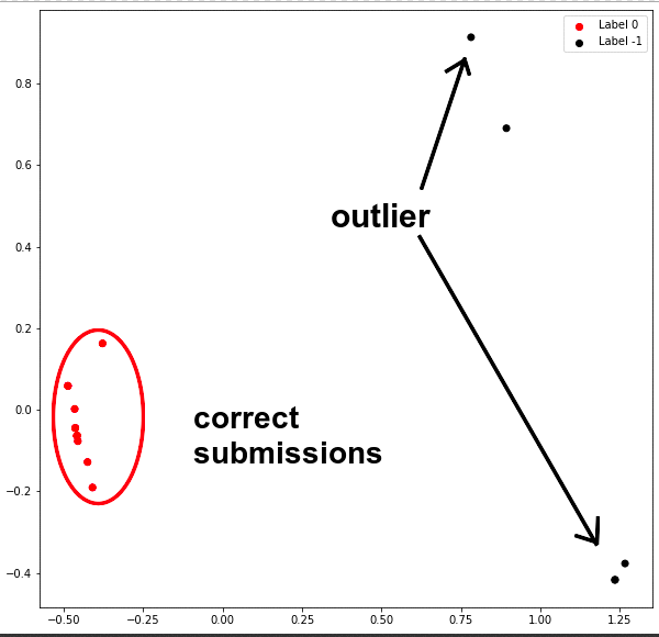
Note: Although it seems like there are fewer than 17 points in the cluster, some of the points in the cluster are below one another.
4. Feature Selection and Tuning Hyperparameters
With any machine learning algorithm, A large part of its implementation involves choosing the correct features and settings.
Setting eps:
The value for eps can then be chosen by using a k-distance graph [1]. This method is slightly tricky to understand but basically, we compute the k-nearest neighbour distances for every point. We then calculate the average of the distances of every point to its k nearest neighbours. Next, these k-distances are plotted in ascending order. The aim is to determine the “knee”, which corresponds to the optimal eps parameter. A knee corresponds to a threshold where a sharp change occurs along the k-distance curve.

In the diagram, the value of eps will correspond to approximately 0.15
Setting min_points:
When Ester [1] first presented DBSCAN in 1996, based on his research he recommended min_points have a default value of 4 (for two-dimensional data).
While Sander [2] suggested setting it to twice the dataset dimensionality, i.e. min_points = (2 . no_of_dimensions).
Selecting clustering features:
Performing cluster analysis on the entire high-level feature set will most probably lead to the Curse of Dimensionality. To reduce the number of features we can employ some standard techniques such as using Correlation among features and Variance Threshold.
If 2 features have a high correlation, this means we can predict one from the other. Therefore, the model only really needs one of them, as the second one does not add additional information. For example, the correlation between mood_happy(happy) and mood_sad(not_sad) should be high and we can remove one of these features.
(Note: Interestingly according to Liem [3] mood_happy(happy) and mood_sad(not_sad) seem to have almost no correlation).
Variance threshold is a simple baseline approach to feature selection. It removes all features whose variance doesn’t meet some threshold. By default, it removes all zero-variance features, i.e., features that have the same value in all samples. Here we assume that features with a higher variance may contain more useful information.
While techniques such as Correlation among features and Variance Threshold will be effective in reducing the number of features, I think the right approach to reducing the dimensions(features )is by standardising the features and then performing Principal Component Analysis. Principal Component Analysis (PCA) is a statistical technique used to reduce the dimensionality of the data (reduce the number of features in the dataset) by selecting the most important features that capture maximum information about the dataset.
The features are selected based on the variance that they cause in the output. Original features of the dataset are converted to the Principal Components which are the linear combinations of the existing features. The feature that causes the highest variance is the first Principal Component. The feature that is responsible for the second-highest variance is considered the second Principal Component, and so on.
Although Principal Components try to cover maximum variance among the features in a dataset, if we don’t select enough Principal Components we may miss some information as compared to the original list of features. Andrew Ng has an interesting video on choosing the Number of Principal Components here
5. High-level Implementation:
This can be divided into 2 parts: A once-off job to cluster all the records already in the database and extending to hl extractor to cluster incoming submissions.
5.1 pseudo-code for Once-off job:
for each MBID in the database:
get all offsets
if number of offsets < minimum number of records required to custer:
    return None
else:
    standardise the data.
    select the first n principal components.
    cluster the submissions.
    store the results of clustering as a JSON (where the offset acts as the key and the value is either 'standard'' or 'outlier' ) in the 'quality' field of the 'info' table.
The minimum number of records needed to perform clustering and the time complexity is dependent on the number of principal components used.
According to Robert [5], the minimum sample size to conduct cluster analysis is 2^m where m is the number of dimensions. However, there seems to be very little research on this and it is a parameter I would like to experiment with.
According to Nidhi (https://doi.org/10.1016/j.procs.2016.07.336) “computational complexity of the whole algorithm is O(n2), where n is the number of degrees (points) in the data set. If effective index structures are used and the dimension of degrees is low (d<=5), the computational complexity of DBSCAN can be reduced to O (n logn ).” Hence we’re looking at between O(n2) and O(n logn ) based on the number of principal components.
5.2 hl extractor:
The hl extractor is a multi-threaded tool used to obtain high-level features from low-level data.
In the main function of acousticbrainz-server/hl_extractor/job_calc.py as soon as the high-level data is obtained and added to the high-level table I plan on calling a function cluster_new_submission(mbid,jdata). This function is responsible for clustering all the new submissions and adding their quality to the info table.
In acousticbrainz-server/hl_extractor/job_calc.py:
try:
    jdata = json.loads(hl_data)
    except ValueError:
    current_app.logger.error("error %s: Cannot parse result document" % mbid)
    current_app.logger.error(hl_data)
    sys.stdout.flush()
    jdata = {}
    db.data.write_high_level(mbid, ll_id, jdata, build_sha1)
"""
parsing the MBID and the JSON containing the high-level data to the cluster function for analysis.
submission_filter is a folder in acousticbrainz-server directory containing the functions required for clustering
"""
    submission_filter.cluster_new_submission(mbid,jdata)
    current_app.logger.info("done %s" % id)
    sys.stdout.flush()
    num_processed += 1
Note 1: unfortunately the process of storing the position of each point in a high dimensional space and recalling it is complex, hence every time a new submission is added we will have to recluster all the data for that MBID.
Note 2: The basic steps in cluster_new_submission(mbid,jdata) would be similar to that of the once-off job.
5.3 Schema changes required:
To integrate this with AcousticBrainz, a new table called quality_info is created.
CREATE TABLE quality_info (
gid UUID NOT NULL,
quality VARCHAR,
recomended_offset INTEGER
);
The gid field acts as the primary key and stores the MBID of a submission.
The quality field is used to store the submission offset and its quality (either outlier or standard ) in the form of a JSON.
Note: For the time being the rocomended_offset column will be null, this will be used later to store the offset of our suggested submission. In the case where there is not enough data to cluster the value of recomended_offset will be -1.
6. Creating the /uuid/info API:
To display the information, I plan on creating at /uuid/info.
The following code will be added to acousticbrainz-server/webserver/views/api/v1/core.py:
@bp_core.route("/<uuid>/info", methods=["GET"])
@crossdomain()
@ratelimit()
def quality_info(mbid):
"""
This endpoint returns a list of all the offsets along if weather it is an outlier or not.
returns
{"mbid1": {"offset1": "standard",
"offset2": "standard",
"mbid2": {"offset1": "outlier",
"mbid_mapping": {"MBID1": "mbid1"}
}
"""
map_classes = _validate_map_classes(request.args.get("map_classes"))
recordings = _get_recording_ids_from_request()
mbid_mapping = _generate_normalised_mbid_mapping(recordings)
recordings = [(mbid, offset) for _, mbid, offset in recordings]

#load_quality_info(recordings, map_classes) featches the quality information from the quality_info table

recording_details = db.data.load_quality_info(recordings, map_classes)
recording_details['mbid_mapping'] = {}
if mbid_mapping:
recording_details['mbid_mapping'] = mbid_mapping
if(recording_details is not None):
return jsonify(recording_details)
return "the data was for this MBID was inconclusive"
7. Timeline:
week 1-2:
Experiment with different features to find the optimum feature and parameters for clustering. These features include min_points, eps(using a k-distance graph ), the number of principal components required (and its effect of runtime) and the minimum number of points required to cluster.
I also want to experiment between principal component analysis vs selecting a subset of features using correlation and variance threshold.
week 3-4:
Focus on implementing the changes required to the hl extractor to cluster new submissions and storing the results of clustering. Develop a mechanism to continuously update the quality_info table when new recordings are added.
week 5-6:
Building the once-off job to cluster records already in the database and testing out the results locally using the data dumps.
week 7-8:
If everything goes according to schedule at this point I want to run the once-off job on the production database.
This period has a lighter workload to account for the time the clustering job will take to run and give me time to fix any bugs and issues that might arise.
week 9-10:
Building /mbid/info API.
Detailed information about me:
Tell us about the computer(s) you have available for working on your SoC project!
I have a Dell Inspiron with an i5 processor and 12GB of ram running Linux.
When did you first start programming?
I began programming with java when I was 15 and I’ve known python for about 2 years now.
What type of music do you listen to?
I love old school rock and pop!
ABBA (d87e52c5-bb8d-4da8-b941-9f4928627dc8)
Queen (0383dadf-2a4e-4d10-a46a-e9e041da8eb3)
Adele (cc2c9c3c-b7bc-4b8b-84d8-4fbd8779e493)
Bryan Adams (4dbf5678-7a31-406a-abbe-232f8ac2cd63)
are some of my favourite artists.
What aspects of the project you’re applying for (e.g., MusicBrainz, AcousticBrainz, etc.) interest you the most?
My favourite aspect of AcousticBrainz is its role in building music recommendation systems. I think music recommendation systems have room for improvement (besides Spotify, most engines recommend artists I already listen to) and AcousticBrainz with its 20 million crowdsourced submissions can be a driving force in building new and better recommendation systems.
Have you ever used MusicBrainz to tag your files?
Yes! I’ve used Picard to tag them.
Have you contributed to other Open Source projects? If so, which projects and can we see some of your code?
Metabrainz is the first open-source organisation I have contributed to with most of my contributions being to ListenBrainz
What sorts of programming projects have you done on your own time?
I love hackathons and the concept of spending 24 hours straight building something amazing!
As part of a hackathon, I built a system to screen patients for Depression using acoustic features of a person’s speech such as pitch, loudness, and speaking rate. ( and we ended up winning the hack!)
I worked on a system that allows patients to store and update their medical records on the cloud and access them using face recognition.
Tried building a system to detect car accidents using the accelerometer in a person’s phone.
How much time do you have available, and how would you plan to use it?
I can dedicate 30 hours a week to GSOC
Do you plan to have a job or study during the summer in conjunction with Summer of Code?
No
Citations
[1] Martin Ester, Hans-Peter Kriegel, Jörg Sander, and Xiaowei Xu. 1996. A density-based algorithm for discovering clusters in large spatial databases with noise. In Proceedings of the Second International Conference on Knowledge Discovery and Data Mining (KDD’96). AAAI Press, 226–231.
[2] Sander, J., Ester, M., Kriegel, HP. et al. Density-Based Clustering in Spatial Databases: The Algorithm GDBSCAN and Its Applications. Data Mining and Knowledge Discovery 2, 169–194 (1998). https://doi.org/10.1023/A:1009745219419
[3] Liem, C. C. S., & Mostert, C. (2020). Can’t trust the feeling? How open data reveals unexpected behavior of high-level music descriptors. In Proceedings of the 21st International Society for Music Information Retrieval Conference (pp. 240-247)
[4] Nidhi and Km Archana Patel. An Efficient and Scalable Density-based Clustering Algorithm for Normalize Data. 2nd International Conference on Intelligent Computing, Communication & Convergence
[5] McClelland, Robert. (2015). Re: What is the minimum sample size to conduct a cluster analysis?. Retrieved from:https://www.researchgate.net/post/What-is-the-minimum-sample-size-to-conduct-a-cluster-analysis/55ff1a97614325339b8b45d6/citation/download.