GSoC 2019: Statistics and data description in AcousticBrainz

[pulkit6559]

Personal information

Name: Pulkit Arora
IRC nick: pulkit6559
Email: pulkitarora7.fas@gmail.com
GitHub: pulkit6559 (Pulkit Arora) · GitHub
Blog: Pulkit Arora – Medium
Time Zone: UTC+0530

Proposal

Summary

AcousticBrainz has, over the years, collected a massive amount of acoustic data from the community. As of now the user doesn’t get much information about this dataset except a plain json list of low-level/high-level data of the recordings. My proposal involves looking at the data present in AcousticBrainz database and providing informative statistics to show to the visitors of AcousticBrainz (also referred as AB) website and the second part involves calculating expectedness of features in a dataset.

Detailed Description

I will be dividing this proposal into 2 sections:

A) Calculating statistics

B) Calculating expectedness of features for each particular track

A) Calculating Statistics

Which statistics to calculate?

Here, the plots have been divided into 2 sections, each divided according to the type of data they represent,

1. General statistics

Here is a list of statistics which can be shown to the users, these stats will be shown on the sitewide statistics page acousticbrainz.org/statistics-graph:

• Recordings - Year bar graph: To show us the yearly distribution of acousticbrainz audio data.
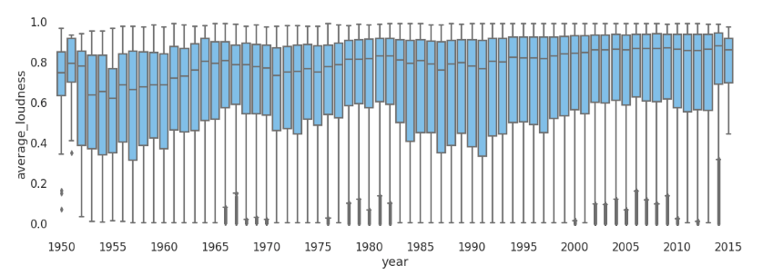
• Feature - Year box plots: These graphs will represent the Feature range (of BPM/average_loudness/danceability/dynamic_complexity/tuning_equal_tempered_deviation) of songs submitted in a particular year and help us visualize any yearly trends followed by them.
  
  
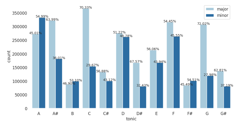
• Keys - count bar graph: To show us the distribution of key values and key scales in the entire audio data.
  
  
• Keys - count bar graph for each genre: To show us the distribution of key values and key scales for each high-level genre.
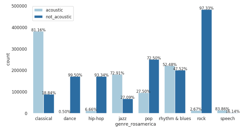
• Mood - genre count bar graphs: For every model, these graphs will help us visualize how a particular mood (acoustic/happy/aggressive/electronic) varies for each genre.
  
  
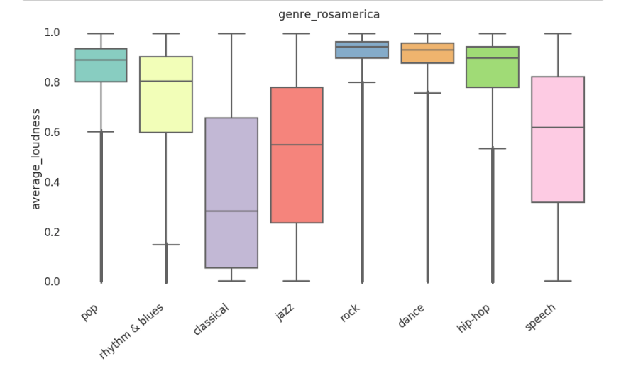
• Feature - Genre box plots: These graphs will allow us to visualize how the average range for a low-level feature (BPM/average_loudness/danceability/chords_change_rate) varies for each genre.
  
  
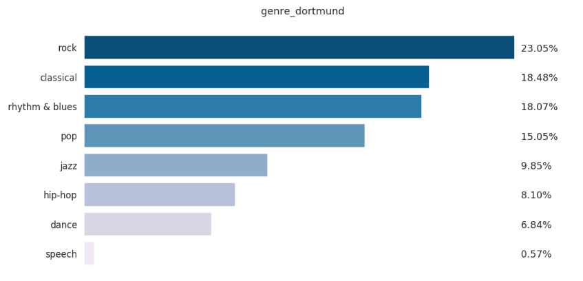
• Pie chart/Bar graph for Genre count/percentage for respective models: For every model, this graph will show the distribution of genre classified by it.
  
  
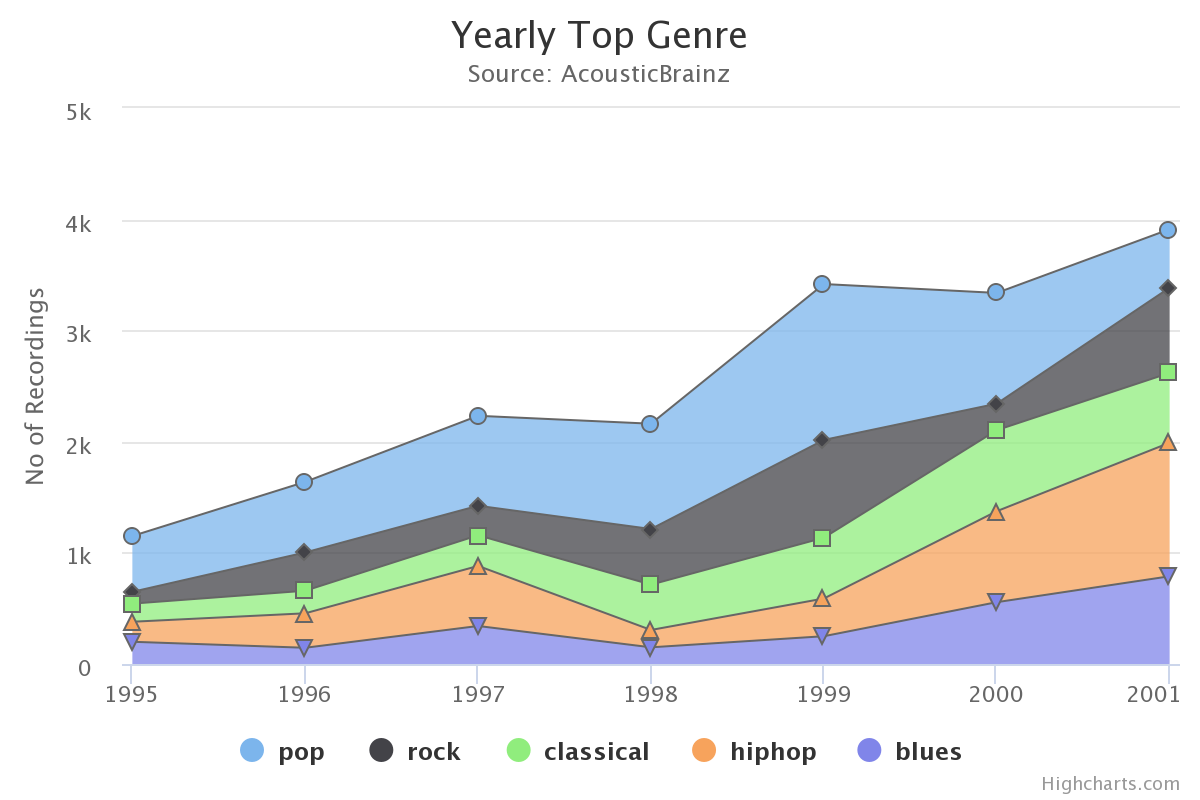
• Year - genre as reported in metadata, this graph will help us visualize how popularity trends for every genre vary for every year.
  
  

The graphs shown above are not an actual representation of how the plots will look like, the actual representations will be created using Highcharts.js

Many of these graphs are taken from acousticbrainz-labs/data-analysis at master · MTG/acousticbrainz-labs · GitHub

Implementation

Whenever a user makes a request to view the AB statistics graph, the flow of data takes the following route:

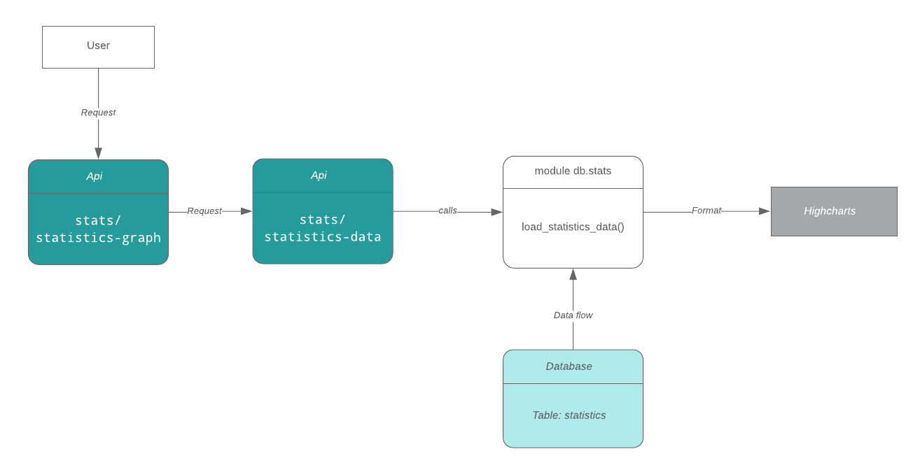
This task will involve addition of two new tables to the AB schema (one to store low-level features and one to store high-level features) for general statistics which would save us the time and effort of extracting and processing json data from existing tables every time a request is made.
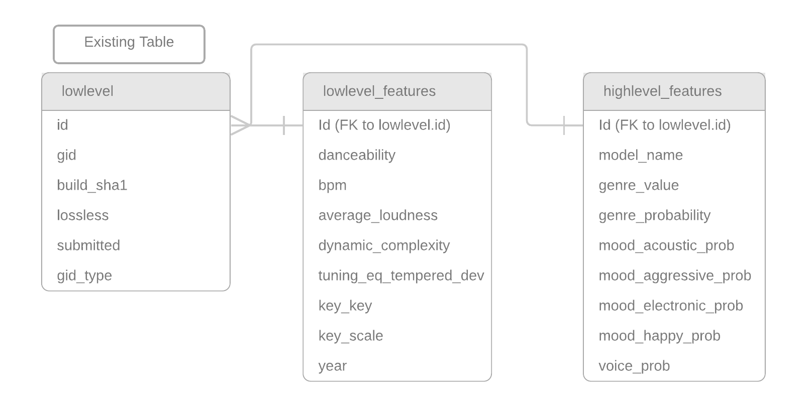
The new tables will contain the following elements:

The new data flow will look something like this

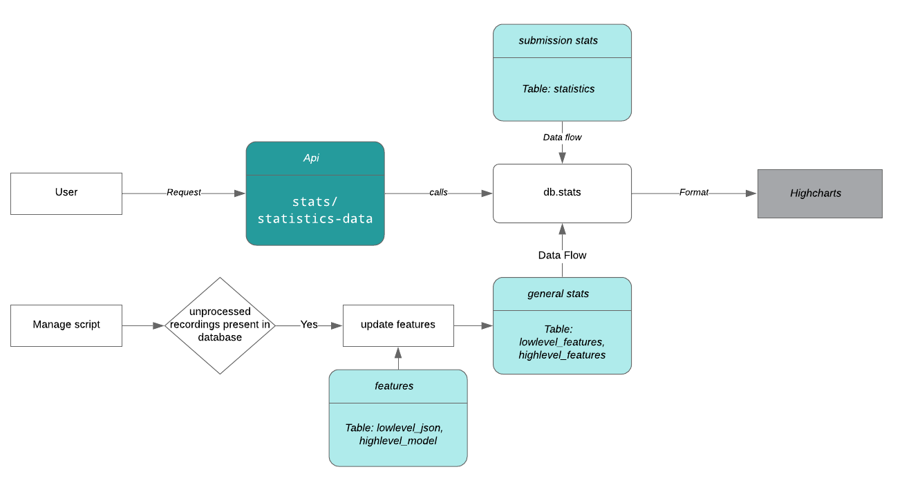
Adding/Updating data in the new tables

Calculation of statistics is a consuming task which requires processing and time, and calculating this data on each request would mean more work for PostgreSQL. On that account, the following steps will ensure the effective calculation of this data.

• To store the audio features which are used to draw plots, we will add two new tables to the schema namely lowlevel_features and highlevel_features
• These tables will populate their rows by extracting data from lowlevel_json and highlevel_model tables respectively.
• For this task a separate script will be written named update_statistics_data which will contain methods to fill and update these tables with low-level and high-level features.
• This script will be run every month through cli commands which will be added to manage.py script using: using: python manage.py compute_stats.
• Since both of these tables contain foreign key ids, pointing to the id field in table lowlevel, data in these tables will be updated using the submitted field.
• Whenever the script update_statistics_data is executed, we will perform a query to determine the latest submitted time up till which the statistics are present.
• Using this submitted time as a reference, we will then query all the recordings which were submitted after this time and extract features from them.

How to render graphs?

To render these graphs, we will use a client-side js plotting library highcharts which provides us with enough tools to create good looking graphs from this data.

Separate API endpoints will be created to query json data from respective tables for each of the above mentioned graphs.

Box/whisker plots showing (feature - year, feature - genre) distributions require a large number of data points to plot especially when we have a large number of outliers, passing all of these values to the client would mean eating up a lot of bandwidth.

Tackling the problem of a large number of outliers

Highcharts provides us a flexible module to create box plots which can be seen here.
It provides us with the option to give an array of 5 values
Eg. [760, 801, 848, 895, 965] where each of these values represents [minimum, lower quartile, median, upper quartile, maximum]
Along with this, we can provide a set of outlier value which can be plotted as a scatter plot for each X.
Therefore, we will calculate these values after querying the data from the tables and instead of sending the long list of json array containing the data points we will show only the smallest and the largest outlier points.

2. Low-level distribution plots

These distribution plots will be calculated for every dataset. For every dataset, classification is done by gaia based on a set of low-level features which can be seen here in the preprocessing yaml file.

The following preprocessings are are done before classification process:

• use all descriptors, no preprocessing
• use lowlevel.* descriptors only
• discard energy bands descriptors (barkbands, energyband, melbands, erbbands)
• use all descriptors, normalize values
• use all descriptors, normalize and gaussianize values

Certain features are always ignored, which include all metadata* that is the information not directly associated with audio analysis. The *.dmean, *.dvar, *.min, *.max, *.cov descriptors are also ignored.

Non-numerical descriptors like (tonal.chords_key, tonal.chords_scale, tonal.key_key, tonal.key_scale), will be enumerated.

We will use these groups of features to draw low-level distribution plots to see if a class has similar values for these features. Since the set features we will be using are multidimensional, we will have to perform some some sort of dimensionality reduction to plot these in 2D space.

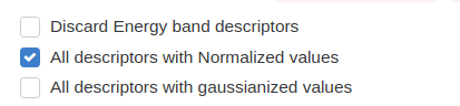
By default we will display plots using only the lowlevel.* descriptors and provide an option to the user to select/un-select these options while sending request for evaluation of 2d plots:

• Discard Energy band descriptors
• All descriptors with Normalized values
• All descriptors with gaussianized and normalized values

This would involve a UI change looking something like:

A separate plot will be shown for each set of these low-level descriptors with values for every class shown with a different color. The graphs will be updated whenever the user requests these graphs to be generated and then stored in the database.

A new react component ‘stats’ will be added alongside view and Evaluation components in datasets view, to show these plots.

Implementation

Fetching low-level features and performing dimensionality reduction on them with every request is impractical, hence the following steps will ensure low fetching time and faster rendering of graphs:

• A separate endpoint will be provided to the author of the dataset called datasets/<uuid>/evaluate_distribution_plots which will create a separate feature matrix containing low-level features of recordings, for each class in the dataset.
• This endpoint will also ensure that the dataset has enough recordings to provide meaningful results (say ~ 100)
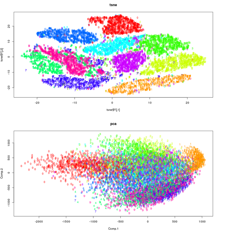
• After the feature matrix is created we will perform dimensionality reduction using either PCA or t-SNE to see which provides visually better results, using dimensionality reduction we will reduce the number of dimensions to 2.
• After these new features are evaluated, the two obtained features are the x and y coordinates of the points of the scatter plot, these coordinates will be evaluated for all sets of features which include (features without energy bands, all features normalized, all features gaussianized and all features normalized and gaussiainized)
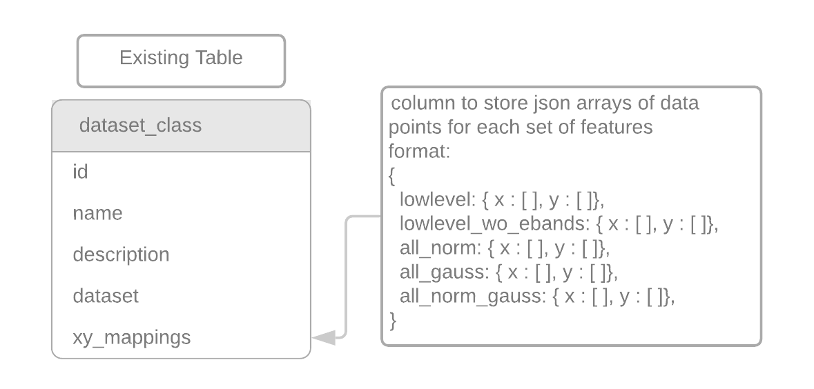
• These x and y coordinates will be stored as json arrays in the table dataset_class in a new column xy_mappings.
  

Viewing distribution plots

To view these plots A react component ‘stats’ will be added alongside view and Evaluation components in datasets view.

Separate endpoints will be created to view these graphs, check boxes will be provided to the user to select one of these set of features:

• features without energy bands,
• all features normalized,
• all features gaussianized and
• all features normalized and gaussiainized

When a particular set of features is selected, the json array of x and y coordinates stored in dataset_class table will be fetched for each class and sent to highcharts.
The graphs drawn will look something like the images shown below, where each color would represent the datapoints of each class

Code Architecture

I intend to create a new sub-package stats in package db which will contain all the scripts responsible for the calculation of statistics and caching frequently used data, this sub-package will contain the following modules:

stats
  ├ tests
  ├ __init__.py
  ├ submission_stats.py (code of statistics.py will be moved here)
  ├ general_stats.py
  └ dataset_lowlevel_distribution.py 

Separate scripts for testing these files will be added in stats/test module

B) Expectedness of features for each particular track

In the datasets present in acousticbrainz, recordings are grouped into 2 or more classes, on these classes, we run svm margin classifiers to calculate percentage accuracy and overlap between them.
After a certain point while adding recordings to the database, we wish to know beforehand whether the recording belongs to the class it is being added in. Such a check will help us create a clear distinction (svm margin) between classes by adding only the recordings whose features lie in a range of expected values, and thus increase the accuracy of the classifier.
The expected values for these classes will be calculated by looking at the low-level data for each group and determining hybrid features best describing the dataset, using methods described in paper: Corpus Analysis Tools for Computational Hook Discover by Jan Van Balen

The order of calculations will be as follows:

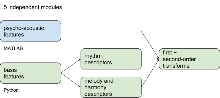
• The code given by jvbalen present on this github repo ‘https://github.com/jvbalen/catchy’ performs feature extraction on given audio data followed by a number of first order and second order transformation, as shown in this flow diagram.
  

  

• However, the low-level data for recordings present in AB database already provides us enough first order features to skip the extraction process and directly perform second order transforms after preprocessing.

• In the paper, the next step involves running PCA on these first and second order features to determine the best group of features which show maximum variation in the data (hence, best representing the data). (*)

• After these features are determined, we find the expected range of values for each of these features [ie. A feature X(i) is normally distributed with mean(u) and standard deviation(sigma)], and for each incoming recording, check if its values lie in this expected range.

• If a recording seems to have values not belonging in the expected range, we show a warning saying “Some of the features of the submitted mbid do not fall in the expected range of values, please make sure the recording is being entered in the correct class”, and leave it on the author if he still wants to submit the recording.

(*) If we wish to not use the hybrid features calculated by pca, and instead compare expectedness of the original low-level features, we can skip this step.
Here is the list of possible features we could use for this task:

  barkbands (mean, var, skewness.mean, skewness.var, kurtosis.mean, kurtosis.var),  
  erbbands (mean, var, skewness.mean, skewness.var, kurtosis.mean, kurtosis.var), 
  gfcc, 
  mfcc,  
  average_loudness, 
  dynamic complexity, 
  bpm, 
  danceability,  
  onset_rate,  
  hpcp (mean, var)

This list is not exhaustive and can be changed after discussions with the mentors and MB community.

How to calculate Second order transforms?

The features which are obtained directly by analyzing the audio files are called First order transforms, we already have these features in the low-level data for each recording, Second order transforms are derivative descriptors that reflect, for a particular feature, how an observed feature value relates to reference data.

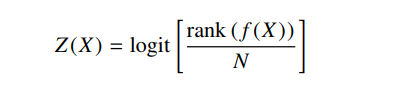
• For 1D features the paper introduces a non-parametric measure of typicality based on log odds. The second-order log odds of a feature value x can be defined as the probability of observing a less extreme value in the reference corpus.
  It can be mathematically represented as:
  
• For 2D features the paper introduced a method based on ranks, Kendall’s rank-based correlation (t), Correlation refers to the association between the observed values of two variables, meaning that as the values for one variable increase, so do the values of the other variable.
  A small code snippet for how these kendall’s correlation coefficients will be calculated is shown below:
  
  

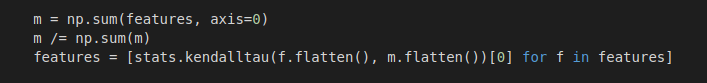
Here, ‘features’ is s 2D ndarray where each row represents one set of values for a feature X(i)

Implementation

• When the user submits a recording id into a class in a dataset, the request will take the following route, each recording will be checked against the expected data stored in ‘dataset_class’ table.
  

  

• Every row in dataset table contains an id which is referenced by its respective class row in dataset_class table. A new column will be added to dataset_class named expected_range which will contain jsonb entities to store mean and standard-deviation of each individual feature for that class.

• These features will be calculated by a new script calc_expected_values.py which will be present in db package. It will contain the code to populate the expected range column using second order transforms on low level features as described above.

• This script will be imported into db/dataset.py which will contain wrapper methods to bind this script, this approach will allow us to work on the calc script separately.

• When new recording Id’s are added to the dataset classes, the wrapper methods in dataset.py will be called to re-evaluate the feature ranges and rewrite the existing expected features with new values.

Timeline

A broad timeline of the work to be done is as follows:

Community Bonding (May 27 - June 24)

During this time, I will Spend this time discussing the points in the proposals and their implementations with my mentors and make any changes if necessary. By, the end of this period I will have a detailed map of what exactly I will code.

Phase 1 (June 25 - July 22)

In this phase I aim to complete subsection (1) of the statistics section, ie. calculating and showing general statistics. This section will involve the addition of new tables to the schema and a new column to the dataset_class table containing coordinates for each recording.

Phase 2 (June 23 - August 19)

In this phase, I aim to complete the UI part of the general statistics. And start with distribution plots for low-level descriptors. Write scripts for calculating and storing mappings into the database and add tests.

Phase 3 (August 1- August 29)

In phase 3, I will finish work on section B and complete the last section of the project ‘ calculating expectedness of features’ after ensuring that the code written in previous phases is clean and tested.

After Summer of Code

I will continue working on AcousticBrainz, after the previous soc’s project on integrating MusicBrainz database into acousticbrainz is merged, work on using mbid redirects to detect duplicate mbids, and using the integration to display artist information.

Here is a more detailed week-by-week timeline of the 13-week GSoC coding period to keep me on track:

PHASE 1

• Week 1: Start by making necessary changes to the AB database schema, and make sure everything is in order with the database to start work on subsequent sections of the project, also start writing scripts for general statistics.
• Week 2: Continue work with general statistics, write queries to load data into the new tables, add cli command to update features.
• Week 3: Write queries to fetch this data to be sent to highcharts.
• Week 4: Work on improving the UI for visualizations added so far, work on tests.

PHASE 2

• Week 5: Fix stuff in the code after mentor evaluations and continue with the next task in hand, i.e., low-level distribution plots.
• Week 6: start working on low-level distribution plots, write the script to process low-level features and produce xy coordinates.
• Week 7: Write endpoints to fetch the coordinates from the database, and work on adding UI for these graphs.
• Week 8: CATCH-UP WEEK: If behind on stuff, then catch up. If not, then continue with section B.

PHASE 3

• Week 9: Fix stuff in the code after evaluation, and continue working with stuff carried on from week 8.
• Week 10: Complete writing script for calculating expected features.
• Week 11: Write queries to store/update and fetch expected values, add tests.
• Week 12: CATCH-UP WEEK: catch up if behind on stuff, finish up with section B.
• Week 13: Pencils down week. Work on final submission and make sure that everything is okay.

Detailed Information about yourself.

I am a sophomore computer science undergrad at MSIT, Delhi, India. I came across AcousticBrainz last year in December, and I have been involved with the development since January. Here is a list of pull requests I have made since then. I intend to revive my old blog to post regular updates about my work in AB throughout the GSoC period.

Question: Tell us about the computer(s) you have available for working on your SoC project!

I have a DELL laptop with an Intel i5 processor and 8 GB RAM, running Ubuntu 18.04.1 LTS.

Question: When did you first start programming?

I have been programming since 11th grade which started as a part of school curriculum, initially wrote some basic programs in c++, followed by a taxi management system using file-handling and data structures. I picked up Java in my freshman year for building some basic android applications and switched to python the same year, since then I’ve been involved with python.

Question: What type of music do you listen to?

Answer: As such I don’t have a type of music I like, but some of the songs I like off the top of my head are: Say Goodbye by Chris Brown, Time Of Our Lives by Pitbull & Ne-Yo, Waiting For The End by Linkin Park.

Question: What aspects of AcousticBrainz interest you the most?

AcousticBrainz is a huge open source repository for acoustic data, there are other projects which facilitate data extraction from audio files, but AB provides us with a database of preprocessed audio data at one single search of its api, along with that the submission process is made very simple by picard.

Question: Have you ever used MusicBrainz to tag your files?

Yes, I have been using Picard to tag my files.

Question: Have you contributed to other Open Source projects? If so, which projects and can we see some of your code?

I have primarily contributed to AcousticBrainz, other than that I submitted a small patch to sympy last year, I have worked on some personal projects on github.

Question: What sorts of programming projects have you done on your own time?

I have worked on implementing various machine learning algorithms in octave and python the code for which can be found here, a movie corpus based chatbot, a miniature version of pacman as a part of college curriculum and currently I’m working on a snakeeyes game which runs on docker and allows users to play online by placing bets and accepting payments, all of which can be found on my github handle.

Question: How much time do you have available, and how would you plan to use it?

I have holidays during most of the coding period and can work full time (45-50 hrs per week) on the project.

Question: Do you plan to have a job or study during the summer in conjunction with Summer of Code?

None, if selected for GSoC.

[pulkit6559]

Hi everyone!, this is an initial draft of my proposal, i’m openly looking for feedbacks and suggestions. : )

[alastairp]

Thanks for your proposal. This is a really exciting project that we’ve wanted in AcousticBrainz for a long time.
Before going any further I want to point out a few things that we’ve already done regarding data display:

• Our original blog post analysing AB data soon after we launched
• Recent work that we’ve done to recreate these graphs in more detail

You should use these examples to give a specific list of what graphs you want to generate. Note that the graphs that we want to show should rely on data that is specifically generated in AcousticBrainz. For example, your graph “Top 3 popular artists” doesn’t make sense in AcousticBrainz, as it doesn’t use any audio features. Please also try and suggest some other graphs that we haven’t made yet. Take a look at the lowlevel and highlevel data that we generate and see if some of these features can be used in graphs. Feel free to talk to us in IRC or in a separate thread if you want to talk about ideas first before integrating them into this proposal.

Be sure about how much work you think that you can complete in the timeline of SoC. We gave an example of 3 subtasks in our ideas list, but this is a lot of work. We would be much happier to see a good, detailed proposal for a smaller number of tasks instead of a brief proposal for a large number of tasks.

I’ll make some comments on the statistics task, but will wait for you to choose which of the other subtasks you would prefer to do and fill it in with more information.

@pulkit6559

1. General statistics

Please make a list of all graphs that you want to show on this page. You’ve only given 1 example graph that uses lowlevel data, and none that use high level data. There are more examples in the links that I gave. Make sure you describe what kind of graph you will use for each data type. Some of your examples could be improved with a different type of graph. For example, consider using box/whisker plots for BPM/year graphs.

@pulkit6559

2. Low-level distribution plots

This section deserves a lot more detail. Have a look into the preprocessing that we perform during model generation. This shows the possible combinations of low-level features that we use when trying to work out the best set of parameters to use to build a model. It makes sense to use these groupings of features to show the graphs because we want to find visual methods of seeing if a class has similar values for a feature. Make an explicit list of the features or groups of features that you will use. Don’t finish this list with ‘etc’ because it seems like you’ve not thought of all possible examples.
The graph that you’ve included in this section doesn’t make sense. you should find a better way of representing the data. Try and build a graph for this proposal using some real data from AcousticBrainz instead of generating fake data.

@pulkit6559

3. Pie charts for various moods

I don’t understand why this section is here. Our mood values themselves are generated by highlevel models. We shouldn’t use this data in relation to new datasets that people are making. Instead, we should use the results of the highlevel models in the graphs in your section 1.

@pulkit6559

This project will involve addition of a new table to the AB schema for general statistics which would save us the time and effort of extracting and processing json data from existing tables every time a request is made.

This is the most important part of this project after choosing the actual graphs to display.

@pulkit6559

For General statistics, I propose the addition of a new table to the schema named general_statistics which would populate its rows by extracting data from lowlevel_json table.

How will this table be populated? (will there be a script to run?) How often will it be run? How will it update existing data?

@pulkit6559

The table will contain the following elements:

I don’t understand how this table structure will work. What graphs can be used by this data? What is the process if I want to add a new graph? How do I get new data into this table? What if the data that I want to show doesn’t relate to year in any way (e.g. genre or key estimation?

@pulkit6559

Frequently used data will be stored in Redis.

What is frequently used data? Please give more detail about how you’ll use redis.

What tools will you use to show the graphs? I see that you’ve given examples using highcharts, but does this support all of the kinds of graphs that you want to show?

@pulkit6559

These stats will be calculated at the end of each month i.e. A 30-day interval, and stored with a time-stamp until next calculation.

@pulkit6559

Optional: Instead of recalculation of stats every time a recording is added, we can create a separate queue for unprocessed recordings, process these on a click of an evaluate button and then empty the queue.

I don’t understand these two comments. It’s not clear when you’ll compute the statistics. The first comment seems to indicate that you’ll do it once a month, but the second one implies that you’re planning on doing it every time a recording is added to acousticbrainz? You need to be clearer about the data flows that you wish to perform. If you’re not sure about the best way to do this then please ask us (in IRC or in a separate forum thread). We’d be happy to help to you define the best way of doing these steps in order to make a better proposal.

[pulkit6559]

Thank you for the review :), using the points you mentioned i have made certain changes to how the stats will be calculated and what kind of graphs will be displayed, i also tried to address the issue i faced regarding the rendering of graphs.
Also, i have decided to drop which was initially the section C of the proposal, considering it was too much work for gsoc period.
Looking forward to your feedback

[alastairp]

Thanks for updating this proposal. There are a few small things that I’d like to be clarified a bit further:

@pulkit6559

This task will involve addition of two new tables to the AB schema (one to store low-level features and one to store high-level features)

Can you clarify this? I’m not sure if you are suggesting that we duplicate all of the data in acousticbrainz in a separate table, or if these tables just store summary information. Duplicating all 11 million rows that we have in AB currently will not be much faster than retrieving the data from the JSON documents. We should have a series of tables that store only summary information. For example, for highlevel features I think we should have a table with these columns:

• model_name
• model_data
• most_recent_submission

So most_recent_submission could have the date of the most recently processed highlevel submission - so that we can update this data with new submissions periodically. The model_data field can be a jsonb field which contains the data directly needed to draw the graph, e.g. {"rock": 100, "jazz": 350, "classical": 20}

We’ll have to work out a way of storing data for items for which we want the quartiles in the data. I had a quick search and it seems like this might be possible: quantiles - Online estimation of quartiles without storing observations - Cross Validated, but we should check how good the results are. There is also a suggestion to use “Reservoir sampling”, which we could do, storing only 100 or 1000 representative samples (e.g. of the loudness for year x). Alternatively, it might make more sense to calculate this data from scratch once a month or so.

@pulkit6559

I intend to create a new sub-package stats in package db which will contain all the scripts responsible for the calculation of statistics and caching frequently used data, this sub-package will contain the following modules:

This is OK, but don’t worry too much about specific implementation details in the proposal. It would be better to have a series of expected data flow diagrams (like you did with your dataflow.png example) showing the general flow of data instead of file and method names. The style of the list of bullet points that you have under the " Adding/Updating data in the new tables" heading is good.

@pulkit6559

By default we will display plots using only the lowlevel.* descriptors and provide an option to the user to select/un-select these options while sending request for evaluation of 2d plots:

I think we should just have an option to choose the preprocessing method out of the 5 methods in the project template. The default option for a model can be the method that was selected by the classifier. For the models in AcousticBrainz you can get the value from the .param file in the models archive

@pulkit6559

To view these plots A react component ‘stats’ will be added alongside view and Evaluation components in datasets view.

Keep in mind that we currently have two types of datasets in AcousticBrainz, the default ones in the model table (and are used to generate highlevel data), and ones made in the dataset editor (we’ve not yet merged them). I think that this part of the project should only deal with the first models.

@pulkit6559

After the feature matrix is created we will perform dimensionality reduction using either PCA or t-SNE to see which provides visually better results, using dimensionality reduction we will reduce the number of dimensions to 2.

I’d like to see this as a specific item in your timeline, I think it’s important enough to be something that you’ll spend some time on

@pulkit6559

B) Expectedness of features for each particular track

This section is pretty good in general, although I’m not sure you’re going to manage to complete all of it in only the third phase. I’d like you to try and split it into 2 equal sized sections so that if you don’t have time to do everything, you can at least do one part of it.
It would be good to see some rough ideas about how you might want to visualise this data in the dataset editor (your “show alert” box in the data flow diagram)

@pulkit6559

Week 4: Work on improving the UI for visualizations added so far, work on tests.

Tests are an integral part of development and shouldn’t be an afterthought on the last week of a phase. Remove this part so that it’s clear that you’ll be writing tests throughout the whole programme!

@pulkit6559

Week 5: Fix stuff in the code after mentor evaluations

Development will work in much the same way that your existing patches have been submitted - so your feedback will come as you submit pull requests, rather than only twice at the evaluation periods. I don’t think you need this part.

@pulkit6559

I have holidays during most of the coding period and can work full time (45-50 hrs per week) on the project.

A typical full-time position (at least in Europe) is 35-40 hours a week. We’d prefer that you put in only 40 hours and do a good job than try and fill up 50 hours and get burned out. Please consider revising this

---

Thanks again for the proposal, and good luck with the submission.